 Image from Wikimedia Commons
Working with MultiIndex and Pivot Tables in Pandas and Python
22 Apr 2018Table of Contents
Here we’ll take a look at how to work with MultiIndex or also called Hierarchical Indexes in Pandas and Python on real world data. Hierarchical indexing enables you to work with higher dimensional data all while using the regular two-dimensional DataFrames or one-dimensional Series in Pandas.
The data set we will be using is from the World Bank Open Data which we can access with the wbdata module by Oliver Sherouse via the World Bank API. To see how to work with wbdata and how to explore the available data sets, take a look at their documentation. Let’s say we want to take a look at the Total Population, the GDP per capita and GNI per capita for each country. We can load this data in the following way.
import matplotlib.pyplot as plt
plt.style.use('ggplot')
import pandas as pd
import wbdata
%matplotlib inline

countries = ['ES', 'FR', 'DE', 'GB', 'IT']

indicators = {'SP.POP.TOTL':'Population',
              'NY.GDP.PCAP.PP.CD':'GDP per capita',
              'NY.GNP.PCAP.PP.CD':'GNI per capita'}

df = wbdata.get_dataframe(indicators=indicators, country=countries)
df.head()
| GDP per capita | GNI per capita | Population | ||
|---|---|---|---|---|
| country | date | |||
| Germany | 2017 | NaN | NaN | NaN |
| 2016 | 48860.525292 | 4.098523e+12 | 82487842.0 | |
| 2015 | 47810.836011 | 3.977536e+12 | 81686611.0 | |
| 2014 | 47092.488372 | 3.888973e+12 | 80982500.0 | |
| 2013 | 45232.197853 | 3.730249e+12 | 80645605.0 |
This already gives us a MultiIndex (or hierarchical index). A MultiIndex enables us to work with an arbitrary number of dimensions while using the low dimensional data structures Series and DataFrame which store 1 and 2 dimensional data respectively. Before we look into how a MultiIndex works lets take a look at a plain DataFrame by resetting the index with reset_index which removes the MultiIndex. Additionally we want to convert the date column to integer values.
df.reset_index(inplace=True)
df['date'] = df['date'].astype(int)
df.head()
| country | date | GDP per capita | GNI per capita | Population | |
|---|---|---|---|---|---|
| 0 | Germany | 2017 | NaN | NaN | NaN |
| 1 | Germany | 2016 | 48860.525292 | 4.098523e+12 | 82487842.0 |
| 2 | Germany | 2015 | 47810.836011 | 3.977536e+12 | 81686611.0 |
| 3 | Germany | 2014 | 47092.488372 | 3.888973e+12 | 80982500.0 |
| 4 | Germany | 2013 | 45232.197853 | 3.730249e+12 | 80645605.0 |
df.index
RangeIndex(start=0, stop=340, step=1)
Here we can see that the DataFrame has by default a RangeIndex. However this index is not very informative as an identification for each row, therefore we can use the set_index function to choose one of the columns as an index. We can do this for the country index by df.set_index('country', inplace=True). This would allow us to select data with the loc function.
How can we benefit from a MultiIndex? If we take a loot at the data set, we can see that we have for each country the same set of dates. In this case it would make sense to structure the index hierarchically, by having different dates for each country. This is where the MultiIndex comes to play. Now, in order to set a MultiIndex we need to choose these two columns by by setting the index with set_index.
df.set_index(['country', 'date'], inplace=True)
df.head()
| GDP per capita | GNI per capita | Population | ||
|---|---|---|---|---|
| country | date | |||
| Germany | 2017 | NaN | NaN | NaN |
| 2016 | 48860.525292 | 4.098523e+12 | 82487842.0 | |
| 2015 | 47810.836011 | 3.977536e+12 | 81686611.0 | |
| 2014 | 47092.488372 | 3.888973e+12 | 80982500.0 | |
| 2013 | 45232.197853 | 3.730249e+12 | 80645605.0 |
That was it! Now let’s take a look at the MultiIndex.
df.index.summary()
'MultiIndex: 340 entries, (Germany, 2017) to (Italy, 1950)'
df.index.names
FrozenList(['country', 'date'])
We can see that the MultiIndex contains the tuples for country and date, which are the two hierarchical levels of the MultiIndex, but we could use as many levels as there are columns available. We can take also take a look at the levels in the index.
df.index.levels
FrozenList([['France', 'Germany', 'Italy', 'Spain', 'United Kingdom'], [1950, 1951, 1952, 1953, 1954, 1955, 1956, 1957, 1958, 1959, 1960, 1961, 1962, 1963, 1964, 1965, 1966, 1967, 1968, 1969, 1970, 1971, 1972, 1973, 1974, 1975, 1976, 1977, 1978, 1979, 1980, 1981, 1982, 1983, 1984, 1985, 1986, 1987, 1988, 1989, 1990, 1991, 1992, 1993, 1994, 1995, 1996, 1997, 1998, 1999, 2000, 2001, 2002, 2003, 2004, 2005, 2006, 2007, 2008, 2009, 2010, 2011, 2012, 2013, 2014, 2015, 2016, 2017]])
Using the MultiIndex
We saw how the MultiIndex is structured and now we want to see what we can do with it. In order to access the DataFrame via the MultiIndex we can use the familiar loc function. (As an overview on indexing in Pandas take a look at Indexing and Selecting Data)
df.loc['Germany', 2000]
GDP per capita    2.729377e+04
GNI per capita    2.228952e+12
Population        8.221151e+07
Name: (Germany, 2000), dtype: float64
We can also slice the DataFrame by selecting an index in the first level by df.loc['Germany'] which returns a DataFrame of all values for the country Germany and leaves the DataFrame with the date column as index.
df_germany = df.loc['Germany']
df_germany.head()
| GDP per capita | GNI per capita | Population | |
|---|---|---|---|
| date | |||
| 2017 | NaN | NaN | NaN |
| 2016 | 48860.525292 | 4.098523e+12 | 82487842.0 |
| 2015 | 47810.836011 | 3.977536e+12 | 81686611.0 |
| 2014 | 47092.488372 | 3.888973e+12 | 80982500.0 |
| 2013 | 45232.197853 | 3.730249e+12 | 80645605.0 |
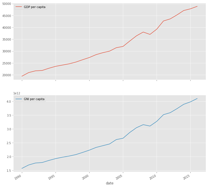
We can use this DataFrame now to visualize the GDP per capita and GNI per capita for Germany.
df_germany[['GDP per capita', 'GNI per capita']].plot(figsize=(12, 12), subplots=True, layout=(2, 1));
Pivot Tables
Now, let’s say we want to compare the different countries along their population growth. One way to do so, is by using the pivot function to reshape the DataFrame according to our needs. In this case we want to use date as the index, have the countries as columns and use population as values of the DataFrame. This works straight forward as follows.
df_pivot = df.reset_index()
df_pivot = df_pivot.pivot(index='date', columns='country', values='Population')
df_pivot.head()
| country | France | Germany | Italy | Spain | United Kingdom |
|---|---|---|---|---|---|
| date | |||||
| 1950 | 42600338.0 | 68376002.0 | 46366767.0 | 28069737.0 | 50616012.0 |
| 1951 | 42809772.0 | 68713920.0 | 46786118.0 | 28236442.0 | 50631571.0 |
| 1952 | 43123100.0 | 69086530.0 | 47171699.0 | 28427994.0 | 50706811.0 |
| 1953 | 43501503.0 | 69483349.0 | 47522671.0 | 28637153.0 | 50829901.0 |
| 1954 | 43916298.0 | 69897556.0 | 47841004.0 | 28858741.0 | 50991454.0 |
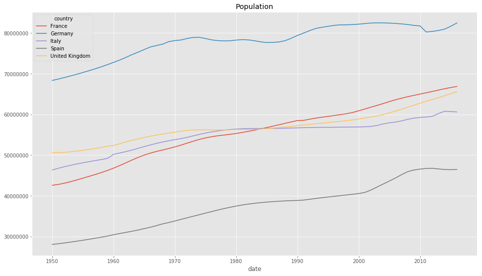
Important to note is that if we do not specify the values argument, the columns will be hierarchcally indexed with a MultiIndex. With this DataFrame we can now show the population of each country over time in one plot
df_pivot.plot(figsize=(16, 9), title='Population');

# Show y-axis in 'plain' format instead of 'scientific'
plt.ticklabel_format(style='plain', axis='y')
Conclusion
We took a look at how MultiIndex and Pivot Tables work in Pandas on a real world example.
You can also reshape the DataFrame by using stack and unstack which are well described in Reshaping and Pivot Tables. For example df.unstack(level=0) would have done the same thing as df.pivot(index='date', columns='country') in the previous example. For further reading take a look at MultiIndex / Advanced Indexing and Indexing and Selecting Data which are also great resources on this topic. Another great article on this topic is Reshaping in Pandas - Pivot, Pivot-Table, Stack and Unstack explained with Pictures by Nikolay Grozev.