 Image from New Old Stock
Working with Pandas Groupby in Python and the Split-Apply-Combine Strategy
18 Mar 2018Table of Contents
In this tutorial we will cover how to use the Pandas DataFrame groupby function while having an excursion to the Split-Apply-Combine Strategy for data analysis. The Split-Apply-Combine strategy is a process that can be described as a process of splitting the data into groups, applying a function to each group and combining the result into a final data structure.
The data set we will be analysing is the Current Employee Names, Salaries, and Position Titles from the City of Chicago, which is listing all their employees with full names, departments, positions, and salaries. Let’s get into it!
%matplotlib inline

import pandas as pd
import matplotlib.pyplot as plt
plt.style.use('ggplot')

path = 'data/Current_Employee_Names_Salaries_and_Position_Titles.csv'
df = pd.read_csv(path)
df.head()
| Name | Job Titles | Department | Full or Part-Time | Salary or Hourly | Typical Hours | Annual Salary | Hourly Rate | |
|---|---|---|---|---|---|---|---|---|
| 0 | AARON, JEFFERY M | SERGEANT | POLICE | F | Salary | NaN | 101442.0 | NaN |
| 1 | AARON, KARINA | POLICE OFFICER (ASSIGNED AS DETECTIVE) | POLICE | F | Salary | NaN | 94122.0 | NaN |
| 2 | AARON, KIMBERLEI R | CHIEF CONTRACT EXPEDITER | GENERAL SERVICES | F | Salary | NaN | 101592.0 | NaN |
| 3 | ABAD JR, VICENTE M | CIVIL ENGINEER IV | WATER MGMNT | F | Salary | NaN | 110064.0 | NaN |
| 4 | ABASCAL, REECE E | TRAFFIC CONTROL AIDE-HOURLY | OEMC | P | Hourly | 20.0 | NaN | 19.86 |
Let’s take a look at what types we have in our DataFrame.
df.info(memory_usage='deep')
<class 'pandas.core.frame.DataFrame'>
RangeIndex: 33183 entries, 0 to 33182
Data columns (total 8 columns):
Name                 33183 non-null object
Job Titles           33183 non-null object
Department           33183 non-null object
Full or Part-Time    33183 non-null object
Salary or Hourly     33183 non-null object
Typical Hours        8022 non-null float64
Annual Salary        25161 non-null float64
Hourly Rate          8022 non-null float64
dtypes: float64(3), object(5)
memory usage: 11.6 MB
On a sidenote, memory_usage='deep' gives us the accurate memory usage of the DataFrame, but it can be slower to load for large DataFrames.
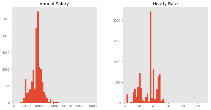
Now lets see what the average Annual Salary and Hourly Rate is by using the DataFrame.mean function. (Note that NaN values are ignored). And while we’re at it, let’s take a look at a histogram of them both with the built-in DataFrame.hist function.
print('Average annual salary : {:8.2f} dollars'.format(df['Annual Salary'].mean()))
print('Average hourly rate   : {:8.2f} dollars'.format(df['Hourly Rate'].mean()))

df[['Annual Salary', 'Hourly Rate']].hist(figsize=(12, 6), bins=50, grid=False);
Average annual salary : 86787.00 dollars
Average hourly rate   :    32.79 dollars
Additionally, we want to convert some of the columns into categorical data, which will reduce the memory usage and speed up the computations in general (unless there are too many categories in a column). We can do this with DataFrame.astype by converting each column seperately or in one step by passing a dictionary with all columns that we want to convert.
# Convert for one column
department = df['Department'].astype('category')

# Convert in one step
df = df.astype({'Department': 'category',
                'Job Titles': 'category',
                'Full or Part-Time': 'category',
                'Salary or Hourly': 'category'})
df.info(memory_usage='deep')
<class 'pandas.core.frame.DataFrame'>
RangeIndex: 33183 entries, 0 to 33182
Data columns (total 8 columns):
Name                 33183 non-null object
Job Titles           33183 non-null category
Department           33183 non-null category
Full or Part-Time    33183 non-null category
Salary or Hourly     33183 non-null category
Typical Hours        8022 non-null float64
Annual Salary        25161 non-null float64
Hourly Rate          8022 non-null float64
dtypes: category(4), float64(3), object(1)
memory usage: 3.4 MB
Introducing Group By
Let’s consider you want to see what the average annual salary is for different departments. For this use case we can take advantage of the DataFrame.groupby function, which is similar to the common GROUP BY statement in SQL.
group = df.groupby('Department')
group
<pandas.core.groupby.DataFrameGroupBy object at 0x7f3e633bb278>
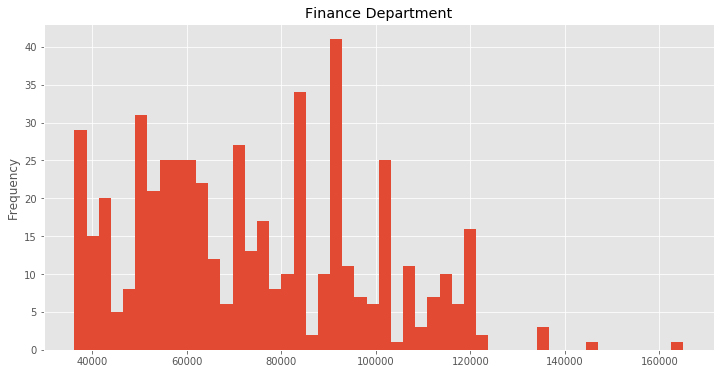
This returns us a DataFrameGroupBy object which is our original DataFrame splitted into multiple DataFrames for each department. We can now get the DataFrame for the finance department and calculate the average annual salary there and use the same DataFrame to create another histogram.
finance_df = group.get_group('FINANCE')
print('Average annual salary in finance department : {:.2f} dollars'.format(
        finance_df['Annual Salary'].mean()))

finance_df['Annual Salary'].plot(kind='hist', bins=50, figsize=(12, 6), title='Finance Department');
Average annual salary in finance department : 73781.26 dollars
Of course you could have done that by simply querying the DataFrame for the finance department with df[df['Department'] == 'FINANCE'], so what is the use of grouping the DataFrame then?
Split-Apply-Combine
By using the groupby method, we are effectively splitting our DataFrame into multiple groups. We can then use these groups to apply various functions to each group to combine them in the end into a final data structure.
This overall process is commonly referred as split-apply-combine, a method similar to MapReduce, which is well described in the pandas documentation and in this paper. We have already covered splitting and in the next step , the apply step, we have various options to consider. We can aggregate information from each group, such as group sums, means, minimum, maximum and others. We can transform each group, such as standardizing or normalizing the values within the group. And finally we can filter groups, by discarding specific groups or filtering the data within each group.
Let’s continue with a simple aggregation function by calculating the mean annual salary for each department. All we need to do is to take our previous groupby object and simply apply the meanfunction.
group = df.groupby('Department')
group.mean().head()
| Typical Hours | Annual Salary | Hourly Rate | |
|---|---|---|---|
| Department | |||
| ADMIN HEARNG | NaN | 78683.692308 | NaN |
| ANIMAL CONTRL | 19.473684 | 66197.612903 | 24.780000 |
| AVIATION | 39.597967 | 78750.549324 | 35.633909 |
| BOARD OF ELECTION | NaN | 53548.149533 | NaN |
| BOARD OF ETHICS | NaN | 95061.000000 | NaN |
This returns us a DataFrame with columns as the average value within each department for all numerical columns in the DataFrame. We can combine multiple functions by the agg function, which gives us a column for each aggregation function and returns again a DataFrame.
group.agg(['count', 'min', 'max', 'std', 'mean']).head()
| Typical Hours | Annual Salary | Hourly Rate | |||||||||||||
|---|---|---|---|---|---|---|---|---|---|---|---|---|---|---|---|
| count | min | max | std | mean | count | min | max | std | mean | count | min | max | std | mean | |
| Department | |||||||||||||||
| ADMIN HEARNG | 0 | NaN | NaN | NaN | NaN | 39 | 41640.0 | 156420.0 | 21576.503446 | 78683.692308 | 0 | NaN | NaN | NaN | NaN |
| ANIMAL CONTRL | 19 | 10.0 | 20.0 | 2.294157 | 19.473684 | 62 | 41832.0 | 130008.0 | 18803.042007 | 66197.612903 | 19 | 22.88 | 52.52 | 6.793810 | 24.780000 |
| AVIATION | 1082 | 20.0 | 40.0 | 2.616414 | 39.597967 | 547 | 35004.0 | 300000.0 | 22958.116620 | 78750.549324 | 1082 | 13.00 | 52.18 | 8.025363 | 35.633909 |
| BOARD OF ELECTION | 0 | NaN | NaN | NaN | NaN | 107 | 27912.0 | 133740.0 | 25383.424530 | 53548.149533 | 0 | NaN | NaN | NaN | NaN |
| BOARD OF ETHICS | 0 | NaN | NaN | NaN | NaN | 8 | 73944.0 | 135672.0 | 21660.019232 | 95061.000000 | 0 | NaN | NaN | NaN | NaN |
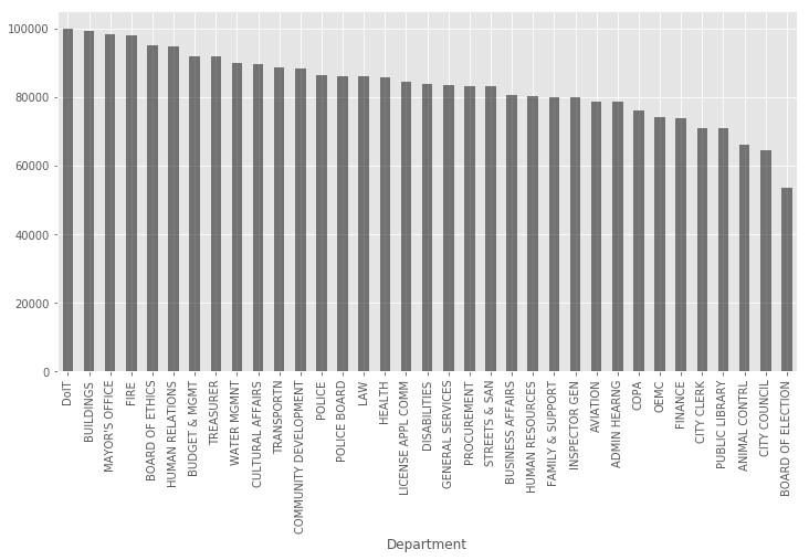
Let’s get back to our question of getting the average annual salary for each department. In order to visualize it properly we are going to make a bar chart with decreasing average annual salary.
group = df.groupby('Department')
average_salary = group['Annual Salary'].mean().sort_values(ascending=False)

# Equivalent way to get average_salary
group = df['Annual Salary'].groupby(df['Department'])
average_salary = group.mean().sort_values(ascending=False)

average_salary.plot(kind='bar', figsize=(12, 6), color='k', alpha=0.5);
Conclusion
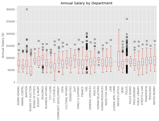
We covered in this tutorial how to work with Pandas Group By function and how to apply the split-apply-combine process to our data set by using various built-in functions. The previously mentioned Pandas documantation and the Pandas Cookbook on grouping covers excelent explanations and advanced examples for split-apply-combine and group by to delve into. As a final bonus, sadly without using group by, here is a way to create a beautiful boxplot of the annual salary by department.
import matplotlib.pyplot as plt

ax = df[['Annual Salary', 'Department']].boxplot(
                by='Department', figsize=(10, 6), rot=90);
ax.set_xlabel('');
ax.set_ylabel('Annual Salary ($)');
ax.set_title('Annual Salary by Department');
plt.suptitle('');  # Getting rid of pandas-generated boxplot title