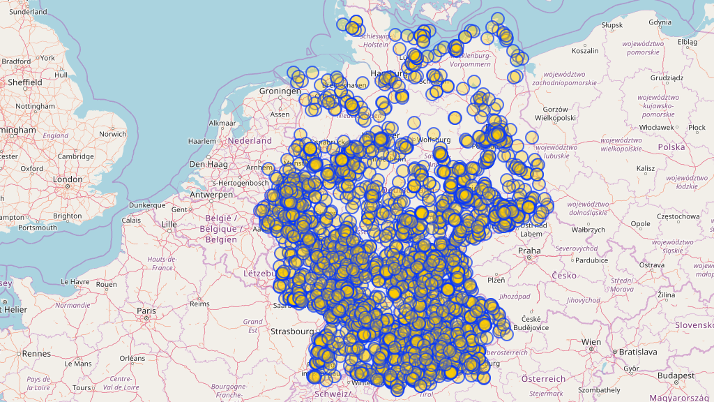
 Image from openstreetmap-heatmap
Loading Data from OpenStreetMap with Python and the Overpass API
04 Mar 2018Table of Contents
Have you ever wondered where most Biergarten in Germany are or how many banks are hidden in Switzerland? OpenStreetMap is a great open source map of the world which can give us some insight into these and similar questions. There is a lot of data hidden in this data set, full of useful labels and geographic information, but how do we get our hands on the data?
There are a number of ways to download map data from OpenStreetMap (OSM) as shown in their wiki. Of course you could download the whole Planet.osm but you would need to free up over 800 GB as of date of this article to have the whole data set sitting on your computer waiting to be analyzed. If you just need to work with a certain region you can use extracts in various formats such as the native .OSM (stored as XML), .PBF (A compressed version of .OSM), Shapefile or GeoJSON. There are also different API possible such as the native OSM API or the Nominatim API. In this article we will only focus on the Overpass API which allows us to select specific data from the OSM data set.
Quick Look at the OSM Data Model
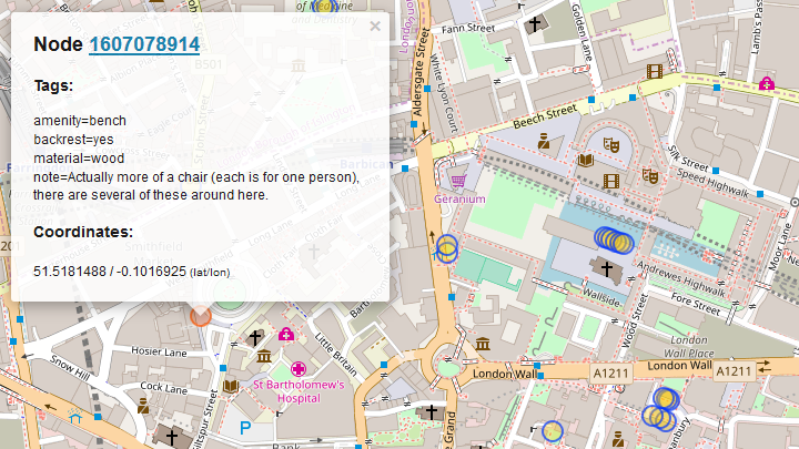
Before we start, we have to take a look at how OSM is structured. We have three basic components in the OSM data model, which are nodes, ways and relations which all come with an id. Many of the elements come with tags which describe specific features represented as key-value pairs. In simple terms, nodes are points on the maps (in latitude and longitude) as in the next image of a well documented bench in London.
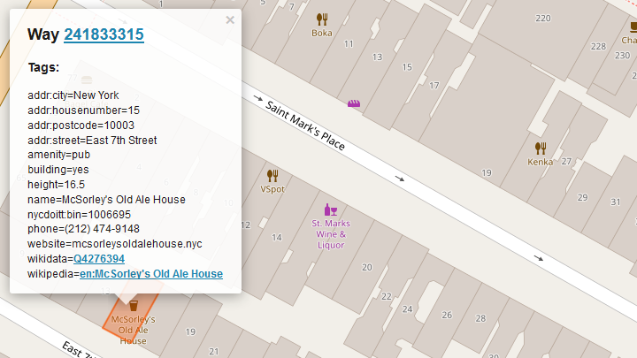
A way on the other hand is a ordered list of nodes, which could correspond to a street or the outline of a house. Here is an example of McSorley’s Old Ale House in New York which can be found as a way in OSM.
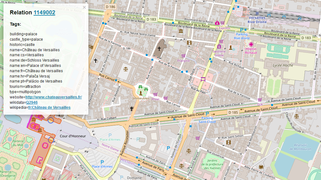
The final data element is a relation which is also an ordered list containing either nodes, ways or even other relations. It is used to model logical or geographic relationships between objects. This can be used for example for large structures as in the Palace of Versailles which contains multiple polygons to describe the building.
Using the Overpass API
Now we’ll take a look how to load data from OSM. The Overpass API uses a custom query language to define the queries. It takes some time getting used to, but luckily there is Overpass Turbo by Martin Raifer which comes in handy to interactively evaluate our queries directly in the browser. Let’s say you want to query nodes for cafes, then your query looks like
node["amenity"="cafe"]({{bbox}}); out;
where each statement in the query source code ends with a semicolon. This query starts by specifying the component we want to query, which is in this case a node. We are applying a filter by tag on our query which looks for all the nodes where the key-value pair is "amenity"="cafe". There are different options to filter by tag which can be found in the documentation. There is a variety of tags to choose from, one common key is amenity which covers various community facilities like cafe, restaurant or just a bench. To have an overview of most of the other possible tags in OSM take a look at the OSM Map Features or taginfo.
Another filter is the bounding box filter where {{bbox}} corresponds to the bounding box in which we want to search and works only in Overpass Turbo. Otherwise you can specify a bounding box by (south, west, north, east) in latitude and longitude which can look like
node["amenity"="pub"]
  (53.2987342,-6.3870259,53.4105416,-6.1148829);
out;
which you can try in Overpass Turbo. As we saw before in the OSM data model, there are also ways and relations which might also hold the same attribute. We can get those as well by using a union block statement, which collects all outputs from the sequence of statements inside a pair of parentheses as in
( node["amenity"="cafe"]({{bbox}});
  way["amenity"="cafe"]({{bbox}});
  relation["amenity"="cafe"]({{bbox}});
);
out;
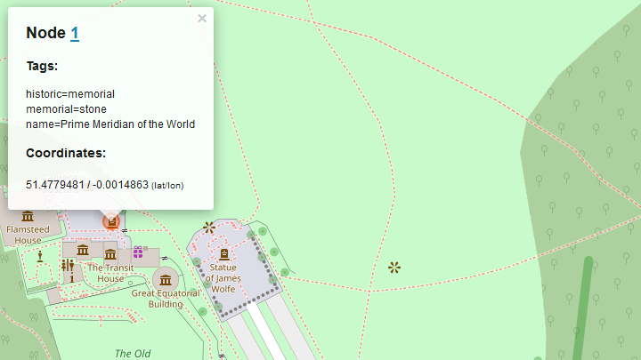
The next way to filter our queries is by element id. Here is the example for the query node(1); out; which gives us the Prime Meridian of the World with longitude close to zero.
Another way to filter queries is by area which can be specified like area["ISO3166-1"="GB"][admin_level=2]; which gives us the area for Great Britain. We can use this now as a filter for the query by adding (area) to our statement as in
area["ISO3166-1"="GB"][admin_level=2];
node["place"="city"](area);
out;
This query returns all cities in Great Britain. It is also possible to use a relation or a way as an area. In this case area ids need to be derived from an existing OSM way by adding 2400000000 to its OSM id or in case of a relation by adding 3600000000. Note that not all ways/relations have an area counterpart (i.e. those that are tagged with area=no, and most multipolygons and that don’t have a defined name=* will not be part of areas). If we apply the relation of Great Britain to the previous example we’ll then get
area(3600062149);
node["place"="city"](area);
out;
Finally we can specify the output of the queried data, which configured by the out action. Until now we specified the output as out;, but there are various additional values which can be appended. The first set of values can control the verbosity or the detail of information of the output, such as ids, skel, body(default value), tags, meta and count as described in the documentation.
Additionally we can add modificators for the geocoded information. geom adds the full geometry to each object. This is important when returning relations or ways that have no coordinates associated and you want to get the coordinates of their nodes and ways. For example the query rel["ISO3166-1"="GB"][admin_level=2]; out geom; would otherwise not return any coordinates. The value bb adds only the bounding box to each way and relation and center adds only the center of the same bounding box.
The sort order can be configured by asc and qt sorting by object id or by quadtile index respectively, where the latter is significantly faster. Lastly by adding an integer value you can set the maximum number of elements to return.
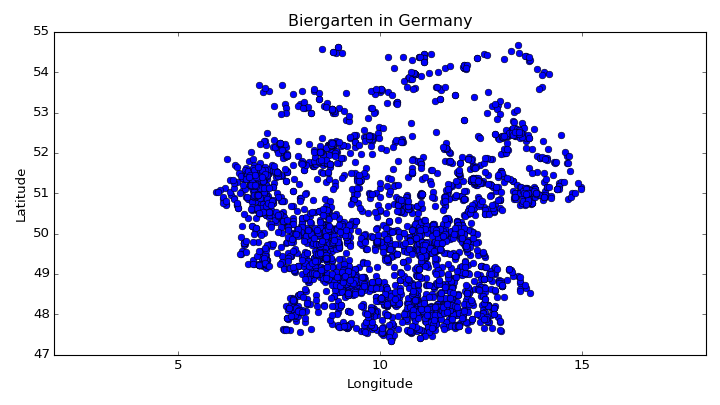
After combining what we have learnt so far we can finally query the location of all Biergarten in Germany
area["ISO3166-1"="DE"][admin_level=2];

( node["amenity"="biergarten"](area);
  way["amenity"="biergarten"](area);
  rel["amenity"="biergarten"](area);
);
out center;
Python and the Overpass API
Now we should have a pretty good grasp of how to query OSM data with the Overpass API, but how can we use this data now? One way to download the data is by using the command line tools curl or wget. In order to do this we need to access one of the Overpass API endpoints, where the one we will look go by the format http://overpass-api.de/api/interpreter?data=query. When using curl we can download the OSM XML of our query by running the command
curl --globoff -o output.xml http://overpass-api.de/api/interpreter?data=node(1);out;
where the previously crafted query comes after data= and the query needs to be urlencoded. The --globoff is important in order to use square and curly brackets without being interpreted by curl. This query returns the following XML result
<?xml version="1.0" encoding="UTF-8"?>
<osm version="0.6" generator="Overpass API 0.7.54.13 ff15392f">
<note>The data included in this document is from www.openstreetmap.org.
      The data is made available under ODbL.</note>
<meta osm_base="2018-02-24T21:09:02Z"/>

  <node id="1" lat="51.4779481" lon="-0.0014863">
    <tag k="historic" v="memorial"/>
    <tag k="memorial" v="stone"/>
    <tag k="name" v="Prime Meridian of the World"/>
  </node>

</osm>
There are various output formats to choose from in the documentation. In order to download the query result as JSON we need to add [out:json]; to the beginning of our query as in
curl --globoff - o output.json http://overpass-api.de/api/interpreter?data=[out:json];node(1);out;
giving us the previous XML result in JSON format. You can test the query also in the browser by accessing http://overpass-api.de/api/interpreter?data=[out:json];node(1);out;.
But I have promised to use Python to get the resulting query. We can run our well known Biergarten query now with Python by using the requests package in order to access the Overpass API and the json package to read the resulting JSON from the query.
import requests
import json

overpass_url = "http://overpass-api.de/api/interpreter"
overpass_query = """
[out:json];
area["ISO3166-1"="DE"][admin_level=2];
(node["amenity"="biergarten"](area);
 way["amenity"="biergarten"](area);
 rel["amenity"="biergarten"](area);
);
out center;
"""
response = requests.get(overpass_url,
                        params={'data': overpass_query})
data = response.json()
In this case we do not have to use urlencoding for our query since this is taken care of by requests.get and now we can store the data or directly use the data further. The data we care about is stored under the elements key. Each element there contains a type key specifying if it is a node, way or relation and an id key. Since we used the out center; statement in our query, we get for each way and relation a center coordinate stored under the center key. In the case of node elements, the coordinates are simply under the lat, lon keys.
import numpy as np
import matplotlib.pyplot as plt

# Collect coords into list
coords = []
for element in data['elements']:
  if element['type'] == 'node':
    lon = element['lon']
    lat = element['lat']
    coords.append((lon, lat))
  elif 'center' in element:
    lon = element['center']['lon']
    lat = element['center']['lat']
    coords.append((lon, lat))

# Convert coordinates into numpy array
X = np.array(coords)

plt.plot(X[:, 0], X[:, 1], 'o')
plt.title('Biergarten in Germany')
plt.xlabel('Longitude')
plt.ylabel('Latitude')
plt.axis('equal')
plt.show()
Another way to access the Overpass API with Python is by using the overpy package as a wrapper. Here you can see how we can translate the previous example with the overpy package
import overpy

api = overpy.Overpass()
r = api.query("""
area["ISO3166-1"="DE"][admin_level=2];
(node["amenity"="biergarten"](area);
 way["amenity"="biergarten"](area);
 rel["amenity"="biergarten"](area);
);
out center;
""")

coords  = []
coords += [(float(node.lon), float(node.lat))
           for node in r.nodes]
coords += [(float(way.center_lon), float(way.center_lat))
           for way in r.ways]
coords += [(float(rel.center_lon), float(rel.center_lat))
           for rel in r.relations]
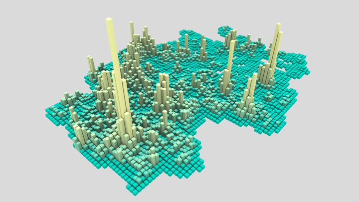
One nice thing about overpy is that it detects the content type (i.e. XML, JSON) from the response. For further information take a look at their documentation. You can use this collected data then for other purposes or just visualize it with Blender as in my openstreetmap-heatmap project.
Conclusion
Starting from the need to get buildings within certain regions, I discovered how many different things are possible to discover in OSM and I got lost in the geospatial rabbit hole. It is exciting to see how much interesting data in OSM is left to explore, including even the possiblity to find 3D data of buildings in OSM. Since OSM is based on contributions, you could also explore how OSM has been growing over time and how many users have been joining as in this article which uses pyosmium to retrieve OSM user statistics for certain regions. I hope I inspired you to go forth and discover curiosities and interesting findings in the depths of OSM with your newly equipped tools.