 Image from Wikimedia Commons
Analyzing Your File System and Folder Structures with Python
23 Jan 2019Table of Contents
- Exploring the File System
- Get Statistics of a File or Directory
- Analyzing Folder Structures
- Conclusion
Say you have an external hard drive with layers upon layers of cryptically named folders and intricate mazes of directories (like here, or here). How can you make sense of this mess? Python offers various tools in the Python standard library to deal with your file system and the folderstats module can be of additional help to gain insights into your file system.
In this article, you will learn the various ways to traverse and explore the file system with Python. In the next section, you will see how to extract statistics from files and directories. In the last section, you will see a practical way to analyze folder structures with folderstats and Pandas with some use cases and visualizations along the way.
Exploring the File System
In Python, you have a number of ways to traverse the file system. The simplest way is by using os.listdir() which lists all filenames and directories in a given folder path. Here is how you can get a list of all files and directories:
import os

folder = '.'
filepaths = [os.path.join(folder, f) for f in os.listdir(folder)]
Note, that you’ll need to get the file path with the os.path.join() function, since os.listdir() only returns the names. You could obviously just combine them with a slash in Linux/macOS or a backslash in Windows, but this function makes sure that the code works platform-independently. To get the absolute file path from a relative path you can additionally use the os.path.abspath() function.
An alternative and faster function is the os.scandir() function (available for Python >= 3.5 or with the scandir module). This function returns an iterator of os.DirEntry objects corresponding to the entries in the directory given by path. The benefit of this function is that you can get file and folder stats with the os.DirEntry object which means less I/O overhead. Here is an example how to get the file paths and directory paths in a directory:
filepaths = [f.path for f in os.scandir('.') if f.is_file()]
dirpaths  = [f.path for f in os.scandir('.') if f.is_dir()]
If you want to get all files and directories recursively, you can do that with the os.walk() function, which generates the file names in a directory tree by walking the tree either top-down or bottom-up. In code this would look like:
for (dirpath, dirnames, filenames) in os.walk('.'):
    for f in filenames:
        print('FILE :', os.path.join(dirpath, f))
    for d in dirnames:
        print('DIRECTORY :', os.path.join(dirpath, d))
Keep in mind that as with os.listdir(), you iterate over each file name, which means that you have to join the directory path dirpath with the file name or directory name. It is also possible to walk the file tree bottom up by adding the argument topdown=False to the os.walk() function. As of Python 3.5, the os.walk() function uses os.scandir() in the background to increase the speed quite significantly. You can read in the article by Ban Hoyt about his story how this was added to the Python standard library.
Another module that you can use to traverse the file system is the glob module. It uses the Unix style pathname pattern expansion, commonly referred to as glob patterns which you would use when working with Linux/macOS. Two common patterns are * which matches with 0 or more arbitrary characters and ? which matches with a single arbitrary character. Additionally, you can have sets of characters defined within [], like with [0-9] which matches a single number. This might look like regular expressions, but it is more limited. This example with glob.glob() shows how to match all JPEGs in a specific folder:
import glob
filepaths = glob.glob('./assets/*.jpg')
This returns the full (relative) paths, so no need for os.path.join(). Also, note that this function returns the file paths in arbitrary order. If you traverse large directories, you might consider using the glob.iglob() function instead, which returns an iterator. As of Python 3.4, you are able to recursively traverse folder structures with glob.glob() and glob.iglob() by adding the argument recursive=True and by adding the ** pattern to the path. For example glob.glob('src/**/*.py', recursive=True) searches for all Python files recursively in the src directory. You can read into the documentation and into glob programming to get a better understanding of this module.
Finally, there has been an effort to improve file handling in Python and as of Python 3.4, we have the pathlib module with a fairly decent solution. This module provides you with object-oriented filesystems paths which makes the handling of files in Python much more readable and gets rid of using os.path.join() all the time. Here is a simple example that prints all files in a folder:
import pathlib

path = pathlib.Path.home() / 'src'
for p in path.iterdir():
    if p.is_file() and p.suffix == '.py':
        print(p.name)
The same can be done by using the Path.glob() method with one less line:
path = pathlib.Path.home() / 'src'
for p in path.glob('*.py'):
    print(p.name)
This can be also achieved recursively by either adding ** to the pattern as we saw previously with the glob module or by using the Path.rglob() method which does that automatically. This is a very extensive module, so make sure to have a look into the documentation to explore the various methods and functions.
Warning: Always check and test the code properly when modifying the file system with any operation like deleting, renaming, copying, among others. And also keep multiple copies of your important files: “Two is One and One is None”.
Get Statistics of a File or Directory
You can get various interesting information from each file. You can get for example the size of the file, the date when the file was modified, and on some platforms, it is possible to see who owns the file and what permissions there are. Here we will focus on the various timestamps and size of a file.
The os module offers the platform-independent os.stat() function which will be our main character here. The function would perform a (POSIX) stat system call on a Unix system (Linux, MacOS) and on Windows it will try to get what it can while some of the variables are filled with dummy values. If you want to get more detailed information on files in Windows, have a look at the WMI package.
Here is how you would get the statistics of a file:
os.stat('path/to/file')
os.stat_result(st_mode=33204, st_ino=524639, st_dev=2054,
    st_nlink=1, st_uid=1000, st_gid=1000, st_size=80907,
    st_atime=1546091718, st_mtime=1541703802, st_ctime=1541703802)
Here you can see the stat_result object of the file with the various attributes which you would get by running stat path/to/file on a Unix system:
File: filename
  Size: 80907     	Blocks: 160        IO Block: 4096   regular file
Device: 806h/2054d	Inode: 524639      Links: 1
Access: (0664/-rw-rw-r--)  Uid: ( 1000/linux-user)   Gid: ( 1000/linux-user)
Access: 2018-12-29 14:55:18.389486626 +0100
Modify: 2018-11-08 20:03:22.320740870 +0100
Change: 2018-11-08 20:03:22.364738380 +0100
 Birth: -
Let’s go through some of the attributes. The st_size describes the number of bytes by the file. (Note: Folders also have a size, although the size is excluding the files inside). When accessing the timestamps, you will see three types which can mean different things on different platforms. Here is an overview of what they mean:
-
atime: time of last access -
mtime: time of last modification -
ctime: time of last status (metadata) change like file permissions, file ownership, etc. (creation time in Windows)
You might imagine that it might be fairly inefficient to update the atime every time a file is read. This timestamp is by default off in Windows and Linux has a couple of different strategies to deal with this: Two common strategies in Unix based systems are noatime, which never updates atime and relatime, which only updates atime once a limit has passed (e.g. once per day) or if the file was modified since the previous read among others. You can see the current strategy that your system uses by running the mount command. You can explore the workings of the stat attributes here. In order to interpret the st_mode of the os.stat() results, you can use the stat module, but can also use os.path.is*() functions instead (like os.path.isdir()) which work as a wrapper for os.stat().
Analyzing Folder Structures
You have seen how to traverse the file system and how to extract statistics. But how do you get the statistics of a folder structure? To tackle the problem I wrote a little module called folderstats that gets the full folder structure including file and folder statistics. In this article, you will learn how to use the resulting data to gain insights from your file system. The module is available on PyPI which you can simply install it with:
pip install folderstats
The module can be used either as a command-line tool or as a module within a script. This makes it easier to prepare the data set beforehand instead of going through a directory multiple times. To illustrate what you can do with the module, we will take a look at the Pandas repository, which will be also our library of choice for further analysis. To download the repository, you can clone it with this command:
git clone https://github.com/pandas-dev/pandas
To use the command-line tool you can run the following command:
folderstats pandas/ -p -i -v -o pandas.csv
This command will collect the statistics into pandas.csv which can be used for further analysis. To explore the various arguments, you can type folderstats --help, which will list all available arguments including some description alongside. In this case the -i argument makes sure that hidden files (starting with a dot like the .git folder or .gitignore) are ignored, -p includes the id of files and folders and the parent ids which can be used to build a graph and finally -v is responsible for a verbose output for some feedback while running. The following snippet does the same thing as the previous command, but this time you can directly use the resulting Pandas dataframe:
import folderstats

df = folderstats.folderstats('pandas/', ignore_hidden=True)
df.head()
| id | path | name | extension | size | atime | mtime | ctime | folder | num_files | depth | parent | |
|---|---|---|---|---|---|---|---|---|---|---|---|---|
| 0 | 2 | pandas/tox.ini | tox | ini | 1973 | 2019-01-13 20:18:17 | 2019-01-13 20:18:17 | 2019-01-13 20:18:17 | False | NaN | 0 | 1 |
| 1 | 3 | pandas/RELEASE.md | RELEASE | md | 238 | 2019-01-13 20:18:17 | 2019-01-13 20:18:17 | 2019-01-13 20:18:17 | False | NaN | 0 | 1 |
| 2 | 4 | pandas/azure-pipelines.yml | azure-pipelines | yml | 3566 | 2019-01-13 20:18:17 | 2019-01-13 20:18:17 | 2019-01-13 20:18:17 | False | NaN | 0 | 1 |
| 3 | 5 | pandas/test.bat | test | bat | 85 | 2019-01-13 20:18:17 | 2019-01-13 20:18:17 | 2019-01-13 20:18:17 | False | NaN | 0 | 1 |
| 4 | 6 | pandas/environment.yml | environment | yml | 807 | 2019-01-13 20:18:17 | 2019-01-13 20:18:17 | 2019-01-13 20:18:17 | False | NaN | 0 | 1 |
Let’s have a look what we’ve got. The statistics cover the file/folder path, file/folder name and file extension. The size is the actual file or folder size in bytes and atime, mtime, and ctime are the various timestamps that we have covered in the previous section. The folder flag specifies whether this element is a folder, the num_files is the number of files within the folder, and the depth states how many layers of folders the file or folder is. Finally, id and parent are responsible to see the links between files and folders which can be used to create a graph. You will see later in this section how to create such a graph.
Exploring File Distributions and Zipf’s Law
The first thing you could explore is the distribution of files by their file extensions. In this case, we would expect mostly Python script files and possibly some other files for documentation or testing. So let’s have a look.
Note, that most of the visualizations are customized with temporary style sheets (plt.style.context('ggplot')). Have a look into the documentation or this tutorial which describe those fairly well. You can skip those if you want to continue with the default values.
In the first visualization, you will see the distribution sorted by their occurrence. This can be done with the .value_counts() method which returns the counts of unique values in a column:
import matplotlib.pyplot as plt

with plt.style.context('ggplot'):
    df['extension'].value_counts().plot(
        kind='bar', color='C1', title='Extension Distribution by Count');
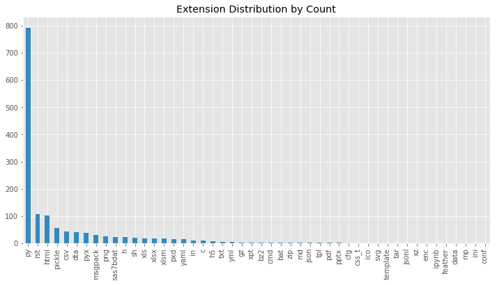
Now, you can see that unsurprisingly the most common file is a .py file responsible for the code which is then followed by .rst and .html files which are both responsible for documentation. It is interesting to see though that there is such a large variety of different file extensions. This showed us only the counts, but what about the sizes? To do this you can use the Pandas .groupby() method to group all extensions (You can read more about groupby in this article). After grouping the files by file extension you can sum all of their sizes:
with plt.style.context('ggplot'):
    # Group by extension and sum all sizes for each extension
    extension_sizes = df.groupby('extension')['size'].sum()
    # Sort elements by size
    extension_sizes = extension_sizes.sort_values(ascending=False)

    extension_sizes.plot(
        kind='bar', color='C1', title='Extension Distribution by Size');
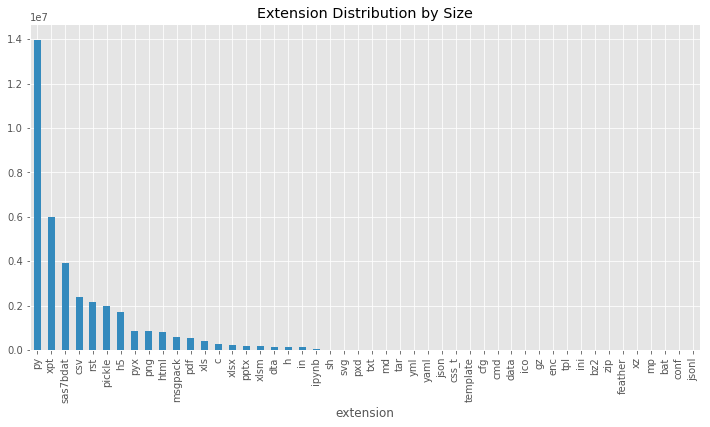
This already gives some interesting insight into the way the files are distributed in the repository. Here we can see that the second largest files are with a .xpt extension, which is SAS transport file used to store data. These files are used for testing. Exploring your file system by size can be very helpful when looking for files or folders that you don’t need, but eat up a lot of memory.
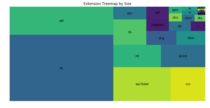
To make this more appealing, let’s use an over-used but nevertheless beautiful Treemap with the squarify module:
import squarify

# Group by extension and sum all sizes for each extension
extension_sizes = df.groupby('extension')['size'].sum()
# Sort elements by size
extension_sizes = extension_sizes.sort_values(ascending=False)

squarify.plot(sizes=extension_counts.values, label=extension_counts.index.values)
plt.title('Extension Treemap by Size')
plt.axis('off');
Next, we can have a look now at the largest folders in the repository. The first thing to do, is to filter the data set to only have folders. The rest should be familiar to the previous visualizations:
with plt.style.context('ggplot'):
    # Filter the data set to only folders
    df_folders = df[df['folder']]
    # Set the name to be the index (so we can use it as a label later)
    df_folders.set_index('name', inplace=True)
    # Sort the folders by size
    df_folders = df_folders.sort_values(by='size', ascending=False)

    # Show the size of the largest 50 folders as a bar plot
    df_sizes['size'][:50].plot(kind='bar', color='C0', title='Folder Sizes');
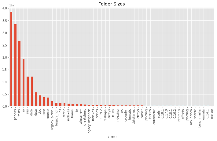
Here you can see that df[df['folder']] filters to have only folders. The first folder without the name is the root folder which has the total size of the folder on your file system.
You might have noticed that most distributions have a similar shape and you might be wondering whether there might be some regularity. Let’s have a quick exploration by plotting the size and rank both in log-scale:
import numpy as np

with plt.style.context('ggplot'):
    y, bins = np.histogram(df['size'], bins=10000)
    plt.loglog(bins[:-1], y, '.');
    plt.ylabel('Size')
    plt.xlabel('Rank')
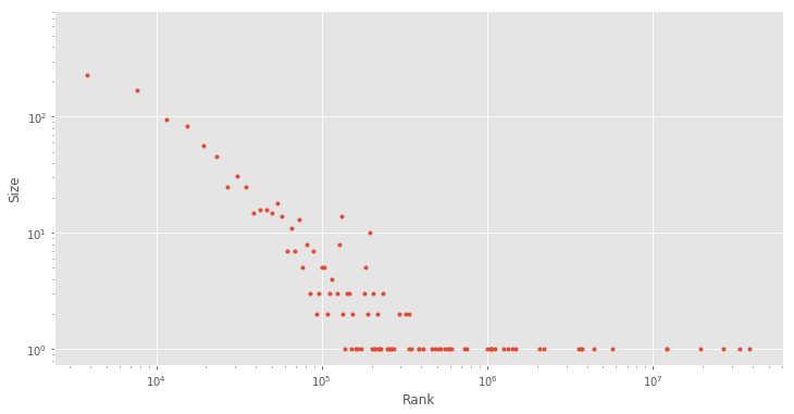
As you can see, this forms a fairly linear relationship between the size and rank. This is surprisingly a very common relationship and it is also known as Zipf’s law (a discrete power law probability distribution), which is a common distribution that is found in most languages:
For example, Zipf’s law states that given some corpus of natural language utterances, the frequency of any word is inversely proportional to its rank in the frequency table. Thus the most frequent word will occur approximately twice as often as the second most frequent word, three times as often as the third most frequent word, etc. (Source)
This is a fascinating distribution that frequently pops up while analyzing language, words, and various different datasets. What’s interesting about this relationship, is that you will see it also fairly often in file systems for some reason. The reason for the occurrence of this relationship is sadly not well understood, but you can explore this topic further in Vsauce’s well made The Zipf Mystery video.
Explore and Visualize the Folder Structure as a Graph
I have promised that the data could be used to analyze the folder structure as a graph. This can be done with the highly extensive NetworkX package. NetworkX is a package that you can use for the creation, manipulation, and analysis of graphs and networks. You have various different data structures, many standard graph algorithms and many other useful features in this context. To get a glimpse of NetworkX, have a look at this tutorial.
Let’s have a look at how we can create a graph from our data set. To build the graph you can iterate over the dataframe and create an edge from row.id to row.parent in the following way:
import networkx as nx

# Sort the index
df_sorted = df.sort_values(by='id')

G = nx.Graph()
for i, row in df_sorted.iterrows():
    if row.parent:
        G.add_edge(row.id, row.parent)

# Print some additional information
print(nx.info(G))
Name:
Type: Graph
Number of nodes: 1656
Number of edges: 1655
Average degree:   1.9988
You can see that we have a total of 1657 nodes (files and folders) and 1656 edges. Since every file and folder can be in only one folder and the first folder has no parent folder, this makes sense. The average degree is the average number of edges that a node can have. Now you could apply all sorts of available Algorithms and Functions to explore and analyze the folder structure, but we will focus on visualizing the graph. NetworkX offers basic functionality for visualizing graphs, but its main focus lies in graph analysis. Here you can see the various drawing tools and libraries that you can use in combination with NetworkX.
In this article, you will see how to work with NetworkX and the Graphviz graph visualization software. Graphviz consists of the DOT graph description language
and a set of tools that can create and process DOT files. Note that you need to have pydot (you can install it with pip install pydot) and Graphviz installed additionally to NetworkX. To see what Graphviz is capable of, have a look at their Gallery.
One visualization layout that you can use is the hierarchical layout with the confusingly similarly named dot tool. Let’s have a look at how that would look like:
from networkx.drawing.nx_pydot import graphviz_layout

pos_dot = graphviz_layout(G, prog='dot')

fig = plt.figure(figsize=(16, 8))
nodes = nx.draw_networkx_nodes(G, pos_dot, node_size=2, node_color='C0')
edges = nx.draw_networkx_edges(G, pos_dot, edge_color='C0', width=0.5)
plt.axis('off');

Great! In the first line you will notice pos_dot = graphviz_layout(G, prog='dot') which is responsible to create the node positions for G using the selected tool (prog='dot') and the graphviz_layout() function. Using these positions, you can draw the nodes with draw_networkx_nodes() function and the edges with draw_networkx_edges() function. In these functions, you have further parameters for more detailed styling.
Perhaps more beautiful, there is the option to use a radial layout using the twopi tool which you can use in the following way:
pos_twopi = graphviz_layout(G, prog='twopi', root=1)

fig = plt.figure(figsize=(14, 14))
nodes = nx.draw_networkx_nodes(G, pos_twopi, node_size=2, node_color='C0')
edges = nx.draw_networkx_edges(G, pos_twopi, edge_color='C0', width=0.5)
plt.axis('off')
plt.axis('equal');

Wonderful! Now you could create a beautiful fractal visualization of your unorganized hard drives and project folders and print it on your wall to remind you to keep your backups up to date. Be aware though, that the time to compute these graph drawing can get quickly out of hand for large graphs (>10000).
Conclusion
You have learned in this article how to deal with your file system in an automated fashion with many of the useful tools in the Python standard library. You have also learned how to analyze folder structures with folderstats and the various ways you can work with the resulting data set. This should prepare you for your next frustrations when dealing with cryptic folder structures and messy file systems.
Here is a list of further reading resources if you want to delve deeper into this topic:
- Diskover: File system crawler, disk space usage, file search engine and file system analytics powered by Elasticsearch
- Contributing os.scandir() to Python
- PEP 471 – os.scandir() function – a better and faster directory iterator
- VSauce - The Zipf Mystery
- NetworkX Tutorial
- NetworkX Examples