Framing Parametric Curves

Table of Contents

• Introduction
• How to describe Curves in Space?
• The Case for Parallel Transport Frames
• Giving the Curve some Surface
• Conclusion

This article explores an efficient way on how to create tubes, ribbons and moving camera orientations based on parametric curves with the help of moving coordinate frames.

Introduction

Before we start we need to understand what a parametric curves is. They are usually described by parametric equations in the form

which are expressed by explicit functions and are parameterized by some variable (\(t\) in this case). In contrast, the corresponding implicit equation to this parametric equation is \(x^2 + y^2 = r^2\), which does not serve us as well for drawing a curve. Parametric equations are commonly packaged and written as vectors in the following form

where \(\overrightarrow{x}\) describes a circle in the plane with radius \(r \in \mathbb{R}\) for the parameter \(t\), giving us a point of a circle for the interval \([0, 1]\). If the equations for this parametric curve are slightly modified and extended, it can lead us to beautiful figures like Lissajous curves or more involved parameterizations like Spirograph figures, Epitrochoids and Hypotrochoids.

How to describe Curves in Space?

Imagine we want to move a camera along a parametric curve in 3D. We cannot just use the sampled points we get from the parametric equations since we have no reference where to look at. Therefore we need to tell the camera in which direction to look and in which direction is “up” along the curve.

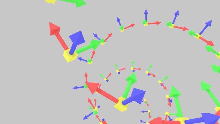
We need a frame of reference, also called moving frame which is moving with the curve and telling us the main directions in the same way that the main coordinate axis tell us the main coordinate directions in \(x, y, z\). Our moving reference frame needs to be also orthonormal (each vector normal to each other) and each vector unit length, which will be useful later on.

A common frame is the Frenet-Serret frame or sometimes referred as simply Frenet frame or TNB frame, which is constructed purely from the velocity and the acceleration of the curve. The velocity is simply described by the first derivative \(\overrightarrow{x}'(t)\) and acceleration by the second derivative \(\overrightarrow{x}''(t)\). The single directions of the frame are then described by the tangential vector \(\overrightarrow{T}\), normal vector \(\overrightarrow{N}\) and binormal vector \(\overrightarrow{B}\) with the following equations.

In many cases we are dealing with sampled points of a curve instead of functions, namely piecewise linear curves (connecting the samples by lines). Therefore we need to calculate the derivatives by means of finite differences. Thus, the tangent vector for each point \(\overrightarrow{x}_i\) of our curve can be calculated by

In the following code snippet you can see the Frenet frame being implemented with Python. To calculate the first and second derivative we apply numpy.gradient to each dimension of our input points, which calculates the finite differences mentioned before. Additionally we apply a lambda function which we use to normalizes the tangent and binormal vectors. Since the binormal and tangent vector are normal to each other and unit vectors, the cross product of them is in turn a normal unit vector.

# Number of points
n = len(points)
	
# Calculate the first and second derivative of the points
dX = np.apply_along_axis(np.gradient, axis=0, arr=points)
ddX = np.apply_along_axis(np.gradient, axis=0, arr=dX)
	
# Normalize all tangents 
f = lambda m : m / np.linalg.norm(m)
T = np.apply_along_axis(f, axis=1, arr=dX)
	
# Calculate and normalize all binormals
B = np.cross(dX, ddX)
B = np.apply_along_axis(f, axis=1, arr=B)
	
# Calculate all normals
N = np.cross(B, T)

So it seems we are done and the Frenet frame solves this problem, but we quickly encounter problems. Consider the following curve

This curve draws a straight-line segment from point \(\overrightarrow{p}\) to point \(\overrightarrow{q}\) for \(t \in [0, 1]\). The first derivative is the vector \(\overrightarrow{x}'(t) = \overrightarrow{q} - \overrightarrow{p}\), but the second derivative is zero. This means it is not possible to calculate the Frenet frame for straight-line segments and at points where the second derivative vanishes. The Frenet frame has also other problems such as ambiguity and sudden orientation changes as we can see here.

The Case for Parallel Transport Frames

An alternative way to define our moving reference frame is illustrated in the publication Parallel Transport Approach to Curve Framing by parallel transporting the frame vectors along a curve. It is based on the observation that the tangential vector \(\overrightarrow{T}(t)\) for a given curve is uniquely defined for each point on the curve. This enables us to choose two perpendicular vectors \(\overrightarrow{U}(t) \perp \overrightarrow{V}(t)\) for the remainder of the curve, as long as the vectors stay in the normal plane perpendicular to \(\overrightarrow{T}(t)\) at each point of the curve. This allows us to transport the normal and binormal vector along without having large orientation changes as in the Frenet frame.

We start the algorithm by calculating all tangential vectors \(\overrightarrow{T_i}\) for all sampled points \(\overrightarrow{x_i}\) and setting an initial normal vector \(\overrightarrow{V_0}\) perpendicular to \(\overrightarrow{T_0}\). For each sampled point we calculate the normal vector \(\overrightarrow{B} \leftarrow \overrightarrow{T_i} \times \overrightarrow{T_{i+1}}\). If the length \(\Vert \overrightarrow{B} \Vert = 0\) (both vectors point in the same direction) then just copy \(\overrightarrow{V_{i+1}} \leftarrow \overrightarrow{V_i}\) otherwise we need to rotate \(\overrightarrow{V_i}\). We do this by first normalizing \(\overrightarrow{B}\) with \(\hat{B} \leftarrow \overrightarrow{B}/\Vert \overrightarrow{B} \Vert\) and calculating the angle between the current and next tangential vector by \(\theta \leftarrow \arccos( \overrightarrow{T_i} \cdot \overrightarrow{T_{i+1}} )\). Using \(\theta\) we can rotate the normal vector by \(\overrightarrow{V_{i+1}} \leftarrow R(\hat{B}, \theta) \overrightarrow{V_i}\), where \(R(\hat{B}, \theta)\) is a rotation matrix defining a rotation around \(\hat{B}\) by angle \(\theta\). The algorithm is implemented in the following snippet with Python

# Number of points
n = len(points)
	
# Calculate all tangents 
T = np.apply_along_axis(np.gradient, axis=0, arr=points)
	
# Normalize all tangents
f = lambda m : m / np.linalg.norm(m)
T = np.apply_along_axis(f, axis=1, arr=T)
	
# Initialize the first parallel-transported normal vector V
V = np.zeros(np.shape(points))
V[0] = (T[0][1], -T[0][0], 0)
V[0] = V[0] / np.linalg.norm(V[0])
	
# Compute the values for V for each tangential vector from T
for i in range(n - 1):
	b = np.cross(T[i], T[i + 1])
	if np.linalg.norm(b) < 0.00001:
		V[i + 1] = V[i]
	else:
		b = b / np.linalg.norm(b)
		phi = np.arccos(np.dot(T[i], T[i + 1]))
		R = rotationMatrix(phi, b)
		V[i + 1] = np.dot(R, V[i])
	
# Calculate the second parallel-transported normal vector U
U = np.array([np.cross(t, v) for (t, v) in zip(T, V)])

If we are dealing with closed curves we want to have the same orientation at the first frame as in the last frame. We can achieve this by slightly rotating our normal vectors \(\overrightarrow{V_i}\) over the course of the curve so the first and the last normal vector have the same orientation.

# Postprocess frames so that first and last frame are the same
if closed:
	theta = np.arccos(np.dot(V[0], V[-1])) / float(n)
	if np.dot(T[0], np.cross(V[0], V[-1])) > 0:
		theta = -theta

	for i in range(n):
		R = rotationMatrix(theta * float(i), T[i])
		V[i] = np.dot(R, V[i])
	
# Calculate the second parallel-transported normal vector U
U = np.array([np.cross(t, v) for (t, v) in zip(T, V)])

Giving the Curve some Surface

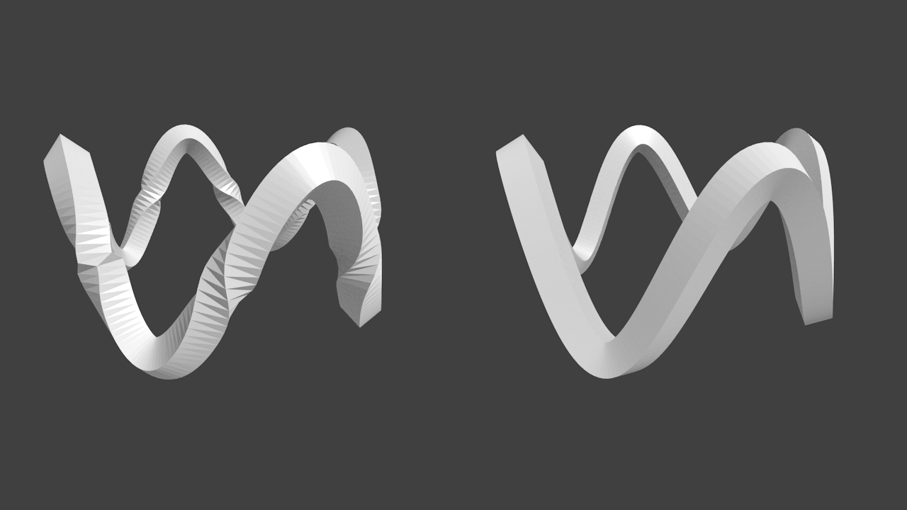
We saw now how to create a moving reference frame for a sampled curve, but now we would like to create a tube along the curve. This can be achieved by defining a parametric surface with the curve points and frames at each point. One way to define such a tube is by a channel surface which is the envelope of a family of spheres of equal radii whose centers are on a given space curve. We can use the following parametric representation of a pipe surface

where \(v \in [0, 1]\) and \(u\) is dictated by our sampling of the curve and \(r\) defines the radius of the tube. The radius can be also defined as a function over \(u\) which grows and shrinks for different \(u\). In the next image we can see such surface parameterizations for the Frenet frame (left) and the parallel transport frame (right). Here we can see the strong orientation changes along the curve for the Frenet frame.

Conclusion

We saw how to create moving reference frames for space curves with the help of the Frenet-Serret frame and the parallel transport frame. Two interesting articles covering the topic for Three.js can be found in the article by @mattdesl. Besides the parallel transport frame approach there are also different approaches such as Rotation Minimizing Frames.