 Image from New Old Stock
Three Ways to get most of your CSV in Python
24 Jun 2017Table of Contents
One of the crucial tasks when working with data is to load data properly. The common way the data is formated is CSV, which comes in different flavors and varying difficulties to parse. This article shows three common approaches in Python.
The data used for the recipes commes from GPSies, a data base of GPS Tracks for hiking, biking and other activities, NYC Department of Transportation with data feeds of New York infrastructure and World Bank Open Data where some data sets like global population of the world can be found.
Load CSV with Python Standard Library
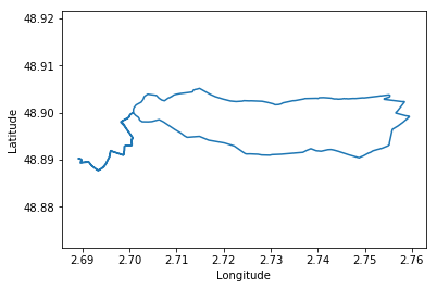
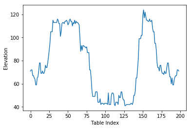
The Python Standard Library offers a wide variety of built-in modules providing system functionality and standardized solutions to common problems. The module we need is the csv module with csv.reader. We will use the data set) of a walking track in France which has the following form
Latitude,Longitude,Elevation
48.89016000,2.689270000,71.0
48.89000000,2.689730000,72.0
48.88987000,2.689810000,72.0
48.88924000,2.689570000,67.0
48.88934000,2.690050000,67.0
48.88949000,2.691400000,65.0
...
We see that the file contains a header and uses commas as delimiters. We can parse this file with
import csv
import numpy as np
import matplotlib.pyplot as plt

data_path = 'data/EntreDhuisEtMarne.csv'
with open(data_path, 'r') as f:
    reader = csv.reader(f, delimiter=',')
    headers = next(reader)
    data = np.array(list(reader)).astype(float)

print(headers)
print(data.shape)
print(data[:3])

# Plot the data
plt.plot(data[:, 1], data[:, 0])
plt.axis('equal')
plt.xlabel(headers[1])
plt.ylabel(headers[0])
plt.show()

plt.plot(data[:, 2])
plt.xlabel('Table Index')
plt.ylabel(headers[2])
plt.show()
['Latitude', 'Longitude', 'Elevation']
(199, 3)
[[ 48.89016   2.68927  71.     ]
 [ 48.89      2.68973  72.     ]
 [ 48.88987   2.68981  72.     ]]
First we need to open the file with open() giving gives us a file object. the with statement makes sure that the file is then closed after the with block. The file is then is used for the csv.reader which can be iterated over all rows returning for each row a list of the items as strings. We then finally transform the data into a Numpy array for further processing.
Load CSV with Numpy
In order to load data with Numpy, you can use the functions numpy.genfromtxt or numpy.loadtxt, where the difference is that np.genfromtxt can read CSV files with missing data and gives you options like the parameters missing_values and filling_values that help with missing values in the CSV. The loading of our data in previous recipe can be done in one step by
data = np.loadtxt(data_path, delimiter=',', skiprows=1)
or with the more powerful nunmpy.genfromtxt
data = np.genfromtxt(datas_path, delimiter=',', names=True)
where the names argument specifies to load the header, which enables us to access the columns with their header names. In this recipe we will load the following data set of the bike racks in NYC
X,Y,Name,small,large,circular,mini_hoop,total_rack
982903.56993819773,205129.99858243763,1 7 AV S,5,0,0,0,5
987330.41607135534,191302.73030526936,1 BOERUM PL,1,0,0,0,1
983210.95318169892,199016.51343409717,1 CENTRE ST,10,0,0,0,10
985897.83954019845,207157.88527469337,1 E 13 ST,1,0,0,0,1
1010993.9694659412,252137.33960694075,1 E 183 ST,0,0,2,0,2
987774.37089210749,210586.44665901363,1 E 28 ST,1,0,0,0,1
...
We can see from the data set that the data types of the columns are mixed. This can be solved by specifying the dtype argument nunmpy.genfromtxt. This can be either a single type like float or a list of formats. These formats are specified by the Data type objects in Numpy.
import numpy as np
import matplotlib.pyplot as plt

data_path = "data/nyc_bike_racks.csv"
types = ['f8', 'f8', 'U50', 'i4', 'i4', 'i4', 'i4', 'i4']
data = np.genfromtxt(data_path, dtype=types, delimiter=',', names=True)

# Plot the data
plt.scatter(data['X'], data['Y'], s=0.5)
plt.axis('equal')
plt.axis('off')
plt.xticks([])
plt.yticks([])

plt.show()

As mentioned before, the names argument enables us to use the header names to select the columns directly with their names as with data['X']. It is important to note that the str data type only works as a data type for all columns and without specified names argument
data = np.genfromtxt(data_path, dtype=str, delimiter=',')
and to skip the header row(s) just add the skip_header=1 argument for the number of rows to be skipped. Additionally numpy.genfromtxt covers functionality for missing values and converters for specific columns.
Load CSV with Pandas
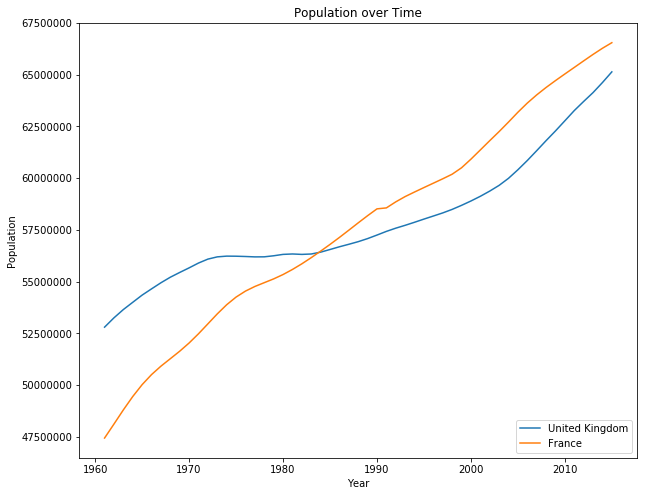
The third and my recommended way of reading a CSV in Python is by using Pandas with the pandas.read_csv() function. The function returns a pandas.DataFrame object, that is handy for further analysis, processing or plotting. In this recipe we will use the more difficult population data set which has the following form:
"Data Source","World Development Indicators",

"Last Updated Date","2017-06-01",

"Country Name","Country Code","Indicator Name","Indicator Code","1960","1961","1962","1963","1964","1965","1966","1967","1968","1969","1970","1971","1972","1973","1974","1975","1976","1977","1978","1979","1980","1981","1982","1983","1984","1985","1986","1987","1988","1989","1990","1991","1992","1993","1994","1995","1996","1997","1998","1999","2000","2001","2002","2003","2004","2005","2006","2007","2008","2009","2010","2011","2012","2013","2014","2015","2016",
"Aruba","ABW","Population, total","SP.POP.TOTL","54208","55435","56226","56697","57029","57360","57712","58049","58385","58724","59065","59438","59849","60239","60525","60655","60589","60366","60106","59978","60096","60567","61344","62204","62831","63028","62644","61835","61077","61032","62148","64623","68235","72498","76700","80326","83195","85447","87276","89004","90858","92894","94995","97015","98742","100031","100830","101218","101342","101416","101597","101936","102393","102921","103441","103889","",
...
First thing we see is that we need to skip some rows to come to the header. Also we want to select Country Code as the index, which will come in handy for selection later on.
import numpy as np
import pandas as pd
import matplotlib.pyplot as plt

path = 'data/population.csv'
df = pd.read_csv(path, skiprows=4)
df = df.set_index('Country Code')
df.head()
| Country Name | Indicator Name | Indicator Code | 1960 | 1961 | 1962 | 1963 | 1964 | 1965 | 1966 | ... | 2008 | 2009 | 2010 | 2011 | 2012 | 2013 | 2014 | 2015 | 2016 | Unnamed: 61 | |
|---|---|---|---|---|---|---|---|---|---|---|---|---|---|---|---|---|---|---|---|---|---|
| Country Code | |||||||||||||||||||||
| ABW | Aruba | Population, total | SP.POP.TOTL | 54208.0 | 55435.0 | 56226.0 | 56697.0 | 57029.0 | 57360.0 | 57712.0 | ... | 101342.0 | 101416.0 | 101597.0 | 101936.0 | 102393.0 | 102921.0 | 103441.0 | 103889.0 | NaN | NaN |
| AFG | Afghanistan | Population, total | SP.POP.TOTL | 8994793.0 | 9164945.0 | 9343772.0 | 9531555.0 | 9728645.0 | 9935358.0 | 10148841.0 | ... | 26528741.0 | 27207291.0 | 27962207.0 | 28809167.0 | 29726803.0 | 30682500.0 | 31627506.0 | 32526562.0 | NaN | NaN |
| AGO | Angola | Population, total | SP.POP.TOTL | 5270844.0 | 5367287.0 | 5465905.0 | 5565808.0 | 5665701.0 | 5765025.0 | 5863568.0 | ... | 19842251.0 | 20520103.0 | 21219954.0 | 21942296.0 | 22685632.0 | 23448202.0 | 24227524.0 | 25021974.0 | NaN | NaN |
| ALB | Albania | Population, total | SP.POP.TOTL | 1608800.0 | 1659800.0 | 1711319.0 | 1762621.0 | 1814135.0 | 1864791.0 | 1914573.0 | ... | 2947314.0 | 2927519.0 | 2913021.0 | 2904780.0 | 2900247.0 | 2896652.0 | 2893654.0 | 2889167.0 | NaN | NaN |
| AND | Andorra | Population, total | SP.POP.TOTL | 13414.0 | 14376.0 | 15376.0 | 16410.0 | 17470.0 | 18551.0 | 19646.0 | ... | 85616.0 | 85474.0 | 84419.0 | 82326.0 | 79316.0 | 75902.0 | 72786.0 | 70473.0 | NaN | NaN |
5 rows × 61 columns
From this table we can see that missing values are automatically included as NaN values. We also can see that an additional column was added to the table, but this is due the commas at the end of each row in the data set. To solve this we can simply drop this column. We now want to plot the populations of France and Great Britain.
# Drop last columns
df.drop(df.columns[-1], axis=1, inplace=True)

# Get all the year columns
year_columns = df.columns[4:]
# Get the years as integer values
years = [int(year) for year in year_columns]

for country in ['GBR', 'FRA']:
    # Get the population for each year
    population = [df.loc[country][year] for year in year_columns]
    # Get the country name
    country_name = df.loc[country]['Country Name']
    # Plot the data
    plt.plot(years, population, label=country_name)

# Add labels
plt.title('Population over Time')
plt.legend(loc='lower right')
plt.xlabel('Year')
plt.ylabel('Population')
plt.ticklabel_format(style='plain')
plt.show()
Here are some good resources for Pandas on Indexing and Selecting Data, Working with Missing Data and Data Structures. There is also a 10 minutes to pandas introduction which covers many helpful use cases.
Conclusion
We have seen three recipes on how to load csv tables in Python with the Python Standard Library, Numpy and Pandas. Each of them is useful in their own way, but for more complex data sets I recommend to work with Pandas. Numpy on the other hand is sufficient for simple homogenous data sets and can be also useful for more involved data sets. Let me know in the comments if you are left with some questions.